Multi-class classification
A two-class classifier can only distinguish two classes, while a multi-class classifier (also called a polynomial classifier) ​​can distinguish more than two classes.
Some algorithms (such as random forest classifier or naive Bayes classifier) ​​can directly deal with multi-class classification problems. Some other algorithms (such as SVM classifier or linear classifier) ​​are strictly binary classifiers. Then, there are many strategies that allow you to perform multi-class classification with a binary classifier.
For example, one way to create a system that can divide pictures into 10 categories (from 0 to 9) is to train 10 binary classifiers, each corresponding to a number (detector 0, detector 1, detector 2, to And so on). Then when you want to classify a picture, let each classifier classify the picture and select the classifier with the highest decision score. This is called the "one-to-one" (OvA) strategy (also called "one-to-one").
Another strategy is to train a binary classifier for each pair of numbers: one classifier is used to process numbers 0 and 1, the other is used to process numbers 0 and 2, the other is used to process numbers 1 and 2, and so on. This is called the "one-to-one" (OvO) strategy. If there are N classes. You need to train N * (N-1) / 2 classifiers. For the MNIST problem, 45 binary classifiers need to be trained! When you want to classify a picture, you must run this picture on all 45 two classifiers. Then see which category wins. The main point of the OvO strategy is that each classifier only needs to be trained on part of the data in the training set. This part of the data is the data corresponding to the two categories that it needs to distinguish.
Some algorithms (such as SVM classifiers) are difficult to expand in the size of the training set, so for these algorithms, OvO is better, because it can be trained more on small data sets, compared to huge data Set speaking. However, for most binary classifiers, OvA is a better choice.
Scikit-Learn can detect that you want to use a binary classifier to complete multi-classification tasks, and it will automatically execute OvA (except for SVM classifier, which uses OvO). Let's try SGDClassifier.
>>> sgd_clf.fit (X_train, y_train) # y_train, not y_train_5 >>> sgd_clf.predict ([some_digit]) array ([5.])
It's easy. The above code trains an SGDClassifier on the training set. This classifier processes the original target class from 0 to 9 (y_train) instead of just detecting whether it is 5 (y_train_5). Then it makes a judgment (there is only one correct number in this case). Behind the scenes, Scikit-Learn actually trained 10 binary classifiers, and each classifier produced a decision value for a picture, and selected the class with the highest value.
To prove that this is true, you can call the decision_function () method. Instead of returning one value for each sample, 10 values ​​are returned, one for each class.
>>> some_digit_scores = sgd_clf.decision_function ([some_digit]) >>> some_digit_scores array ([[-311402.62954431, -363517.28355739, -446449.5306454, -183226.61023518, -414337.15339485, 161855.74572176 ,. -452576.39616962,573,471-, ])
The highest value is corresponding to category 5:
>>> np.argmax (some_digit_scores) 5 >>> sgd_clf.classes_ array ([0., 1., 2., 3., 4., 5., 6., 7., 8., 9.]) >>> sgd_clf.classes [5] 5.0
After a classifier is trained, it will save the list of target categories to its attributes classes_, sorted by value. In this example, the index of each class in the classes_ array conveniently matches the class itself. For example, the class with index 5 happens to be category 5 itself. But usually not so lucky.
If you want to force Scikit-Learn to use OvO strategy or OvA strategy, you can use OneVsOneClassifier class or OneVsRestClassifier class. Create a sample and pass a binary classifier to its constructor. For example, the following code will create a multi-class classifier, using the OvO strategy, based on SGDClassifier.
>>> from sklearn.multiclass import OneVsOneClassifier >>> ovo_clf = OneVsOneClassifier (SGDClassifier (random_state = 42)) >>> ovo_clf.fit (X_train, y_train) >>> ovo_clf.predict ([some_digit]) array ([5. ]) >>> len (ovo_clf.estimators_) 45
Training a RandomForestClassifier is equally simple:
>>> forest_clf.fit (X_train, y_train) >>> forest_clf.predict ([some_digit]) array ([5.])
This time Scikit-Learn does not need to run OvO or OvA because the random forest classifier can directly classify a sample into multiple categories. You can call predict_proba () to get a list of probability values ​​for the corresponding category of the sample:
>>> forest_clf.predict_proba ([some_digit]) array ([[0.1, 0., 0., 0.1, 0., 0.8, 0., 0., 0., 0.]])
You can see that the classifier is pretty sure of its prediction: 0.8 at index 5 of the array, which means that the model estimates that this picture represents the number 5 with an 80% probability. It also thinks that this picture may be the number 0 or the number 3, respectively, are 10% chance.
Now of course you want to evaluate these classifiers. As usual, you want to use cross-validation. Let's use cross_val_score () to evaluate the accuracy of SGDClassifier.
>>> cross_val_score (sgd_clf, X_train, y_train, cv = 3, scoring = "accuracy") array ([0.84063187, 0.84899245, 0.86652998])
It has 84% ​​accuracy on all test folds. If you use a random classifier, you will get 10% accuracy. So this is not a bad score, but you can do better. For example, simply regularizing the input will increase the accuracy to more than 90%.
>>> from sklearn.preprocessing import StandardScaler >>> scaler = StandardScaler () >>> X_train_scaled = scaler.fit_transform (X_train.astype (np.float64)) >>> cross_val_score (sgd_clf, X_train_scaled, y_train, cv = 3, scoring = "accuracy") array ([0.91011798, 0.90874544, 0.906636])
Error Analysis
Of course, if this is an actual project, you will follow the following steps in your machine learning project (see Appendix B): Explore candidates for data preparation, try multiple models, and list the best models Shortlist, debug hyperparameters with GridSearchCV, automate as much as possible, as you did in the previous chapter. Here, we assume that you have found a good model and you try to find ways to improve it. One way is to analyze the type of error produced by the model.
First, you can check the confusion matrix. You need to make a prediction using cross_val_predict (), and then call the confusion_matrix () function, as you did earlier.
>>> y_train_pred = cross_val_predict (sgd_clf, X_train_scaled, y_train, cv = 3) >>> conf_mx = confusion_matrix (y_train, y_train_pred) >>> conf_mx array (([[5725, 3, 24, 9, 10, 49, 50, 10, 39, 4], [2, 6493, 43, 25, 7, 40, 5, 10, 109, 8], [51, 41, 5321, 104, 89, 26, 87, 60, 166, 13] , [47, 46, 141, 5342, 1, 231, 40, 50, 141, 92], [19, 29, 41, 10, 5366, 9, 56, 37, 86, 189], [73, 45, 36, 193, 64, 4582, 111, 30, 193, 94], [29, 34, 44, 2, 42, 85, 5627, 10, 45, 0], [25, 24, 74, 32, 54, 12, 6, 5787, 15, 236], [52, 161, 73, 156, 10, 163, 61, 25, 5027, 123], [43, 35, 26, 92, 178, 28, 2, 223, 82, 5240]])
Here is a pair of numbers. It is more convenient to use Matplotlib's matshow () function to present the confusion matrix as an image.
plt.matshow (conf_mx, cmap = plt.cm.gray) plt.show ()

This confusion matrix looks pretty good, because most of the pictures are on the main diagonal. On the main diagonal means being classified correctly. The grid corresponding to number 5 looks much dimmer than other numbers. This may be that there are few pictures of the number 5 in the data set, or that the classifier does not perform as well for the number 5 as other numbers. You can verify two situations.
Let us focus on the image presentation that contains only error data. First you need to divide each value of the confusion matrix by the total number of pictures in the corresponding category. In this way, you can compare the error rate rather than the absolute number of errors (which is unfair to large categories).
row_sums = conf_mx.sum (axis = 1, keepdims = True) norm_conf_mx = conf_mx / row_sums
Now let's fill the diagonal with 0. In this way, only the misclassified data is retained. Let us draw this result.
np.fill_diagonal (norm_conf_mx, 0) plt.matshow (norm_conf_mx, cmap = plt.cm.gray) plt.show ()

Now you can clearly see the various errors produced by the classifier. Remember: rows represent actual categories, and columns represent predicted categories. Columns 8 and 9 are quite bright, which tells you that many pictures are mistakenly divided into numbers 8 or 9. Similarly, lines 8 and 9 are also quite bright, telling you that the numbers 8, 9 are often mistaken for other numbers. In contrast, some lines are quite black, such as the first line: this means that most of the number 1 is correctly classified (some are misclassified as number 8). Note that the error graph is not strictly symmetrical. For example, there are more numbers that are misclassified as number 8 than the number that misclassified number 8 as number 5.
Analyzing confusion matrices can usually provide you with deep insights to improve your classifier. Looking back at this picture, it looks like you should try to improve the performance of the classifier on numbers 8 and 9, and correct the confusion of 3/5. For example, you can try to collect more data, or you can construct new features that help the classifier. For example, write an algorithm to count closed loops (for example, number 8 has two rings, number 6 has one, and 5 has no). Or you can preprocess the image (for example, use Scikit-Learn, Pillow, OpenCV) to construct a pattern, such as a closed loop.
Analyzing unique errors is a good way to gain insights about how your classifier works and why it fails. But this is relatively difficult and time-consuming. For example, we can draw the numbers 3 and 5
cl_a, cl_b = 3, 5 X_aa = X_train [(y_train == cl_a) & (y_train_pred == cl_a)] X_ab = X_train [(y_train == cl_a) & (y_train_pred == cl_b)] X_ba = X_train [(y_train = = cl_b) & (y_train_pred == cl_a)] X_bb = X_train [(y_train == cl_b) & (y_train_pred == cl_b)] plt.figure (figsize = (8,8)) plt.subplot (221); plot_digits ( X_aa [: 25], ../images_per_row=5) plt.subplot (222); plot_digits (X_ab [: 25], ../images_per_row=5) plt.subplot (223); plot_digits (X_ba [: 25], ../images_per_row=5) plt.subplot (224); plot_digits (X_bb [: 25], ../images_per_row=5) plt.show ()
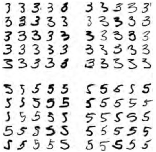
The two 5 * 5 blocks on the left identify the number as 3, and the right identify the number as 5. Some numbers that are misclassified by the classifier (such as the blocks in the lower left and upper right corners) are quite poorly written, and even make it difficult for humans to classify (such as the number 5 in the first column of the 8th row, which looks very like the number 3 ). However, most of the misclassified numbers are obvious errors in our opinion. It is difficult to understand why the classifier is wrong. The reason is the simple SGDClassifier we use, which is a linear model. All it does is assign a class weight to each pixel, and then when it sees a new picture, it adds the weighted pixel intensities, and each class gets a new value. Therefore, because only a small percentage of pixels differ between 3 and 5, this model can easily confuse them.
The main difference between 3 and 5 is the position of the thin line connecting the top line and the bottom line. If you draw a 3 and the connection is slightly shifted to the left, the classifier will probably classify it as 5. vice versa. In other words, this classifier is quite sensitive to the displacement and rotation of the picture. So, one way to reduce the 3/5 confusion is to preprocess the pictures to ensure that they are well centered and not over-rotated. This is also likely to help alleviate other types of errors.
Multi-label classification
So far, all the examples have always been assigned to only one class. In some cases, you may want your classifier to output multiple categories for a sample. For example, consider a face recognizer. If it recognizes several people for the same picture, what should it do? Of course it should put a label on everyone it recognizes. For example, this classifier is trained to recognize three faces, Alice, Bob, Charlie; then when it is input a picture containing Alice and Bob, it should output [1, 0, 1] (meaning: Alice is , Bob is not, Charlie is). This classification system that outputs multiple binary labels is called a multi-label classification system.
At present we do not intend to go deep into facial recognition. We can look at a simple example first, just for the purpose of clarification.
from sklearn.neighbors import KNeighborsClassifier y_train_large = (y_train> = 7) y_train_odd = (y_train% 2 == 1) y_multilabel = np.c_ (y_train_large, y_train_odd) knn_clf = KNeighborsClassifier () knn_label.
This code creates an y_multilabel array that contains two target labels. The first label indicates whether the number is a large number (7, 8 or 9), and the second label indicates whether the number is odd. The next few lines of code will create a sample of KNeighborsClassifier (it supports multi-label classification, but not all classifiers are available), and then we use a multi-target array to train it. Now you can generate a prediction, and then it outputs two labels:
>>> knn_clf.predict ([some_digit]) array ([[False, True]], dtype = bool)
It works correctly. The number 5 is not a large number (False), but also an odd number (True).
There are many ways to evaluate a multi-label classifier, and choose the correct metric, depending on your project. For example, one method is to measure the F1 value for each individual label (or any other two-class classifier measurement standard discussed earlier), and then calculate the average value. The following code calculates the average F1 value of all tags:
>>> y_train_knn_pred = cross_val_predict (knn_clf, X_train, y_train, cv = 3) >>> f1_score (y_train, y_train_knn_pred, average = "macro") 0.96845540180280221
It is assumed here that all tags are of equal importance, but this may not be the case. In particular, if you have more photos of Alice than Bob or Charlie, maybe you want the classifier to have a greater weight on Alice's photos. A simple option is to give each label a weight equal to its support (for example, the number of samples for that label). To do this, simply set average = "weighted" in the above code.
Multi-output classification
The last classification task we will discuss is called "multi-output-multi-class classification" (or simply multi-output classification). It is a simple generalization of multi-label classification, where each label can be multi-category (for example, it can have more than two possible values).
To illustrate this, we build a system that can remove noise from pictures. It takes a picture mixed with noise as input, and expects it to output a clean digital picture, represented by an array of pixel intensities, just like MNIST pictures. Note that the output of this classifier is multi-label (one pixel per label) and each label can have multiple values ​​(pixel intensity values ​​range from 0 to 255). So it is an example of a multi-output classification system.
The line between classification and regression is fuzzy, as in this example. It stands to reason that predicting the intensity of a pixel is more similar to a regression task than a classification task. Moreover, the multi-output system is not limited to classification tasks. You can even let your system output multiple tags for each sample, including class tags and value tags.
Let's start with the MNIST image to create the training set and test set, and then add noise to the pixel intensity of the image. Here is the NumPy's randint () function. The target image is the original image.
noise = rnd.randint (0, 100, (len (X_train), 784)) noise = rnd.randint (0, 100, (len (X_test), 784)) X_train_mod = X_train + noise X_test_mod = X_test + noise y_train_mod = X_train y_test_mod = X_test
Let's take a look at a picture in the test set (yes, we are spying on the test set, so you should immediately Zou Mei):
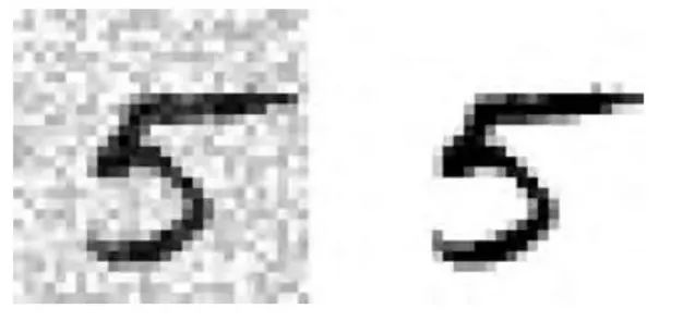
The input picture with noise on the left. On the right is a clean target picture. Now we train the classifier and let it clean this picture:
knn_clf.fit (X_train_mod, y_train_mod) clean_digit = knn_clf.predict ([X_test_mod [some_index]]) plot_digit (clean_digit)
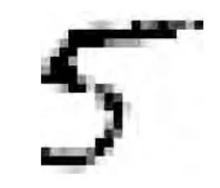
It looks close enough to the target picture. Now summarize our classification journey. I hope you should now know how to choose a good measurement standard, pick a suitable accuracy / recall rate compromise, compare classifiers, and more generally, establish a good classification system for different tasks.
Exercise
Try to build a classifier on the MNIST data set to make it more than 97% accurate on the test set. Tip: KNeighborsClassifier is very suitable for this task. You just need to find a good hyperparameter value (try grid search for weights and hyperparameter n_neighbors).
Writing a function can move the image in MNIST by one pixel in any direction (up, down, left, and right). Then, for each picture on the training set, copy four moved copies (one copy in each direction) and add them to the training set. Finally, train your best model on the expanded training set, and measure its accuracy on the test set. You should observe that your model will perform better. This method of manually expanding the training set is called data augmentation, or training set expansion.
Take the Titanic dataset to tinker. There is a great platform for starting this project: Kaggle!
Create a spam classifier (this is a more challenging exercise):
Download sample data for spam and non-spam. The address is a public dataset of Apache SpamAssassin
Unzip these data sets and become familiar with its data format.
Split the data set into training and test sets
Write a data preparation pipeline to convert each email into a feature vector. Your pipeline should convert a message into a sparse vector. For all possible words, this vector marks which word appears and which word does not appear. For example, if all emails contain only the four words "Hello", "How", "are", "you", then an email (content: "Hello you Hello Hello you") will be converted to Vector [1, 0, 0, 1] (meaning: "Hello" appears, "How" does not appear, "are" does not appear, "you" appears), or [3, 0, 0, 2], if you Want to count the number of occurrences of each word.
You may want to add hyperparameters to your pipeline, control whether to strip the header, convert the message to lowercase, remove punctuation, replace all URLs with "URL", replace all numbers with "NUMBER", or even extract words Do it (for example, truncate the suffix. There are ready-made Python libraries to do this).
Then try a few different classifiers and see if you can build a great spam classifier with high recall and high accuracy.
Capillary Of Thermometer,Bourdon Gauge Thermometer,Capillary In Thermometer,Thermometer Pressure Gauge
ZHOUSHAN JIAERLING METER CO.,LTD , https://www.zsjrlmeter.com